Potentially causal
g lives on h ≥ 0. Temperature now, CO₂ later. This is every row of Table 1 at L = 0.
Koutsoyiannis, Math. Biosci. Eng. 2024
Recreated figures and tables from Demetris Koutsoyiannis’s stochastic causality paper — using the same public reconstructions and instrumental records. At every time span from 500 million years to the last 70, the data say the same thing the “CO₂ drives climate” slogan does not: T → [CO₂], not the reverse.
Graphical abstract · Table 1
Median IRF lag h½ versus analysis time scale. Longer records resolve slower biosphere and ocean mechanisms — they do not reverse who leads.
Log–log recreation of the paper’s summary figure. Each point is one row of Table 1 (causal system T → [CO₂], L = 0).
01
Humans emit CO₂, it accumulates, the greenhouse thickens, temperature follows. Simple. The climate system is not.
02
If [CO₂] caused T, the impulse response would live on negative lags of T → [CO₂] — or the reverse system would win. It does not, on any span the paper can resolve.
03
Change in temperature leads; change in carbon dioxide concentration lags. Unidirectional. Proxy and instrumental. Annual to million-year.
Figure 1–2 · 541 million years
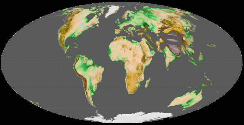
Pangaea · ~200 Ma
Mesozoic supercontinent from the paper’s Figure 1 (Wikimedia, CC BY-SA 4.0). Land–sea geography is itself a climate boundary condition — independent of the modern CO₂ narrative.
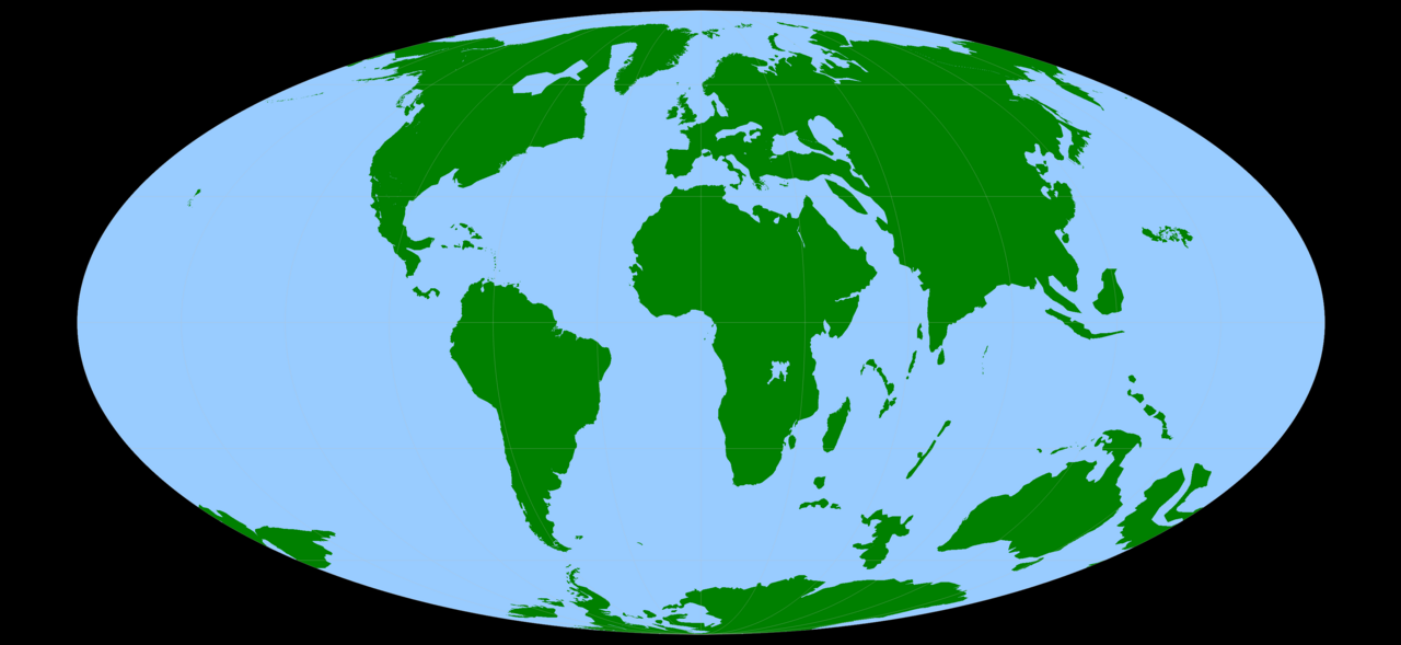
Eocene · ~40 Ma
Continents near modern positions, still no Antarctic ice sheet of today’s size. From the paper’s Figure 1 (Wikimedia, CC BY-SA 4.0).
| Ma BP | Event | Kind |
|---|---|---|
| 485 | Ordovician–Silurian extinction · ~70% genus loss | extinction |
| 372 | Late Devonian extinction · ~35% genus loss | extinction |
| 252 | Permian–Triassic extinction · ~56% genus loss | extinction |
| 201 | Triassic–Jurassic extinction · ~43% genus loss | extinction |
| 66 | Cretaceous–Paleogene extinction · ~40% genus loss | extinction |
| 530 | Animals on land / fish | creation |
| 430 | Land plants, insects | creation |
| 360 | Amphibians | creation |
| 230 | Dinosaurs, first mammals | creation |
| 140 | Flowering plants | creation |
| 60 | Primates | creation |
| 0.3 | Homo sapiens | creation |
Figure 3 · 66 million years
Figure 4 · Vostok ice core · 420 kyr
Figure 5 · last two millennia
Figure 6 · instrumental era
Figures 7–9 · Sections 2.6 & 3
Figure 9 · what the IRF is allowed to mean
An impulse response g(h) says how [CO₂] reacts, h steps after a kick in T. The adverb in the paper is “potentially”: these shapes are necessary, not sufficient. The dashed mark is the mean lag μh.
Potentially causal
g lives on h ≥ 0. Temperature now, CO₂ later. This is every row of Table 1 at L = 0.
Potentially mixed
Mass on both sides, more on the positive. Time order still leans T first.
Hen-or-egg
Symmetric around zero. Two exceptions in Table 1 still have positive characteristic lags.
Potentially anticausal
g lives on h < 0. This is what [CO₂] → T would need. Figure 22 looks like this, and e collapses.
Three questions the paper actually asks
Models, and what they are not
GEOCARB / GEOCARBSULF are box models of weathering and burial, not weather simulators. CENOGRID is a dated δ¹⁸O splice. ERA5 is a reanalysis. Foster 2017 is a proxy ensemble with a LOESS. None of them is the causality test. The test is the IRF on the observations those products emit. Fetch status and original URLs live in Sources & methods.
Berner & Kothavala 2001, Am. J. Sci.
Berner 2006 GCA; Berner 2008 AJS
Royer, Donnadieu, Park, Kowalczyk & Goddéris 2014, Am. J. Sci.
Foster, Royer & Lunt, Nat. Commun. 8:14845
Westerhold et al. 2020, Science; PANGAEA 917503 / 917717
Epstein et al. 1953; as applied in Koutsoyiannis §2.3
Hersbach et al., Copernicus CDS; paper via KNMI Climate Explorer
Morice et al. 2021, JGR Atmospheres; HadCRUT.5.1.0.0
Koutsoyiannis 2020–2024; this paper §3 and Appendix B
Figures 10–22 · the actual test
Vostok original · 416 kyr
Table 1 · every test, one direction
| Case | O/D | Span | Scale | l, m | e causal | e anti | hc | h½ | μh |
|---|---|---|---|---|---|---|---|---|---|
| Phanerozoic | O | 491 Myr | 1 Myr | 1, 1 | 0.62 | 0.61 | 3.0 Myr | 1.2 Myr | 4.0 Myr |
| Phanerozoic | D | 490 Myr | 1 Myr | 1, 1 | 0.27 | 0.19 | 2.0 Myr | 2.3 Myr | 6.4 Myr |
| Cenozoic | O | 66.8 Myr | 100 kyr | 1, 1 | 0.80 | 0.78 | 400 kyr | 760 kyr | 910 kyr |
| Late Quaternary | O | 416 kyr | 1 kyr | 1, 1 | 0.84 | 0.71 | 1 kyr | 1 kyr | 5 kyr |
| Late Quaternary | O | 200.5 kyr | 500 yr | 1, 1 | 0.89 | 0.72 | 2 kyr | 1 kyr | 3 kyr |
| Late Quaternary | D | 200 kyr | 500 yr | 1, 1 | 0.22 | 0.15 | 0 mo | 1 kyr | 2 kyr |
| Common Era | O | 1711 yr | 1 yr | 1, 4 | 0.49 | 0.41 | 35 yr | 25 yr | 33 yr |
| Common Era | O | 1701 yr | 10 yr | 1/10, 4 | 0.49 | 0.40 | 35 yr | 26 yr | 33 yr |
| Common Era | D | 1700 yr | 10 yr | 1/10, 4 | 0.11 | 0.05 | 35 yr | 21 yr | 30 yr |
| Modern / Mauna Loa | D | 63 yr | 1 yr | 1/12, 1 | 0.43 | 0.07 | 7 mo | 7 mo | 8 mo |
| Modern / Mauna Loa | D | 54 yr | 10 yr | 1/120, 1 | 0.49 | 0.38 | 7 mo | 5 mo | 10 mo |
| Modern / Mauna Loa | D | 54 yr | 10 yr | 1/120, 4 | 0.50 | 0.08 | 8 mo | 3.1 yr | 3.2 yr |
| Modern / South Pole | D | 65 yr | 1 yr | 1/12, 1 | 0.30 | 0.03 | 7 mo | 8 mo | 9 mo |
| Modern / South Pole | D | 56 yr | 10 yr | 1/120, 1 | 0.54 | 0.43 | 10 mo | 1.2 yr | 10 mo |
| Modern / South Pole | D | 56 yr | 10 yr | 1/120, 4 | 0.54 | 0.17 | 10 mo | 3.3 yr | 3.3 yr |
Source: Koutsoyiannis 2024, Table 1. Causal lags generally maximize explained variance. Exceptions: (a) Phanerozoic original, L = −14, h½ = 3.7 Myr, μh = 0; (b) Late Quaternary differenced, L = −1, h½ = 850 yr, μh = 1,970 yr. Both still have CO₂ lagging.
Phanerozoic
0.62 vs 0.61
Even the messiest, million-year proxies refuse [CO₂] → T.
Vostok original
0.84 vs 0.71
The textbook ice-core figure, once you stop hiding the lag.
Mauna Loa annual
0.43 vs 0.07
Modern instruments, differenced: anticausal explained variance collapses.
Sections 5–6 · what the figures are for
“No real-world, data-based, evidence has ever been provided in support of that popular speculation. Here evidence of the opposite is provided.”
Data availability · sources & methods
Fetched on first try
33
NOAA GML, HadCRUT5, Vostok NCEI, Moberg, Law Dome 2006, GEOCARB III, the paper itself.
Recovered on retry
7
CENOGRID S34, Royer 2014, Christiansen NOAA, van Hoof EuropePMC, Taylor Dome, Berner 2008.
Still paywalled
4
Shaviv 2023, Grossman 2022, Song 2019 S1, Davis 2017. Curves read from the paper’s figures.
Timed out / dead
5
Scripps Keeling, NASA GISS, CDIAC FTP (530), KNMI ERA5 dump, Etheridge 1996 NOAA path.
Models in play
Two families. Carbon-cycle boxes and proxy stacks reconstruct the deep past. Reanalyses and station files cover the instrumental era. The causality test is not a GCM — it is an impulse-response identification on those series.
Long-term carbon-cycle model
Phanerozoic [CO₂] dashed curve in Figure 2. Weathering, degassing, and burial on a ~10 Myr step. Not a GCM.
Berner & Kothavala 2001, Am. J. Sci.Coupled C–S cycle model
Paper cites Berner 2008. 2006 Geochimica PDF is Elsevier; 2008 volcanic-weathering AJS HTML fetched. 2009 AJS O₂ addendum 404 on the Yale path.
Berner 2006 GCA; Berner 2008 AJSMonte Carlo on GEOCARBSULF
Royer/Davis Phanerozoic [CO₂] compilation lineage. Yale AJS path 404; AJS attachment PDF recovered (1.7 MB).
Royer, Donnadieu, Park, Kowalczyk & Goddéris 2014, Am. J. Sci.Proxy ensemble + LOESS
Phanerozoic [CO₂] in Figure 2. Springer supplementary xlsx 403. PMC HTML fetched; NOAA Paleo-pCO2 holds the 2012 boron file, not the 2017 LOESS product. Plotted curve digitized from the paper.
Foster, Royer & Lunt, Nat. Commun. 8:14845Astronomically tuned benthic splice
Cenozoic −δ¹⁸O. Science Table S34 xlsx 403. PANGAEA parent ?format=html 400. Bare DOI + S34 LOESS textfile (2.3 MB) and MARUM Tables_S8_S34.xlsx recovered. Paper uses ISOBENd18oLOESSsmooth on a 100-kyr step.
Westerhold et al. 2020, Science; PANGAEA 917503 / 917717Visual temperature scale
Converts CENOGRID δ¹⁸O to a °C axis for the plot only. Causality math uses −δ¹⁸O itself.
Epstein et al. 1953; as applied in Koutsoyiannis §2.3Atmospheric reanalysis
Modern T in Figure 6. KNMI static dump 404 (interactive session required). CDS needs an API key. Traces digitized from the paper; HadCRUT5 is the independent instrumental check.
Hersbach et al., Copernicus CDS; paper via KNMI Climate ExplorerIn situ temperature analysis
Not the paper’s series. Shown on Figure 6 as a check, offset +14.35 °C so it sits on the ERA5 absolute axis.
Morice et al. 2021, JGR Atmospheres; HadCRUT.5.1.0.0Transfer-function causality
The actual test. Table 1 is the scoreboard. Characteristic lags grow with window length because g has a heavy tail (Hurst–Kolmogorov), not because the direction flips.
Koutsoyiannis 2020–2024; this paper §3 and Appendix BHow the series were treated
Eras stay on their own clocks. The app never glues monthly Keeling onto ice-core millennia. That is the paper’s Figure 7 argument, enforced in the layout.
Where a named source is paywalled or the tabulated supplement 403s, the plotted series is an axis-calibrated reading of the paper’s own figures (Koutsoyiannis 2024 Figs. 1–6). That is a recreation of what the paper used, not a new compilation.
Treat [CO₂] as the output of a linear filter driven by temperature. Estimate impulse response gⱼ. Potential causality (T → CO₂) puts g on positive lags; explained variance e peaks at computational lag L = 0; the reverse system is anticausal or weak. Characteristic lags: h_c (max cross-correlation), h½ (median of |g|), μ_h (mean of |g|).
Each era panel runs a transparent Pearson cross-correlation on z-scored, interpolated pairs, optionally first-differenced. Positive lag means temperature leads. The IRF gallery (Figs. 11–22) is FIR least squares with ridge, not the paper’s full §3 identifier; Table 1 numbers are transcribed from the paper.
Vostok CO₂ is plotted on gas age (Barnola), not ice age. Enclosure lag is ~2 kyr in warm periods and ~6 kyr in the coldest. Even after that correction, CO₂ still lags deuterium temperature.
Fetch ledger
Original URL first. If it failed, a public mirror. If that failed, the paper’s figure. Status is about the file, not about the science.
Stochastic assessment of temperature–CO₂ causal relationship. Math. Biosci. Eng. 21(7): 6560–6602.
Used: all figures · Table 1 transcribed · Open access, CC BY 4.0. 1.56 MB from NTUA ITIA.
Journal HTML of the same article.
Used: methods text
Appendices plus the graphical-abstract lag figure.
Used: Table 1, hero scatter · Supplement PDF 354 kB; SummaryLags.jpg 830 kB.
Keeling / NOAA GML co2_mm_mlo. Paper’s modern station.
Used: Figure 6 · Text + CSV both 200.
scrippsco2.ucsd.edu in-situ monthly CSV.
Used: unused — NOAA used instead · TCP timeout. Original URL kept.
Failed link kept: https://scrippsco2.ucsd.edu/assets/data/atmospheric/stations/in_situ_co2/monthly/monthly_in_situ_co2_mlo.csv
Surface flask 1° CCGG monthly.
Used: Figure 6
Surface in-situ CCGG monthly.
Used: archive · Trends path gml.noaa.gov/webdata/ccgg/trends/co2/co2_mm_spo.txt is 404.
scrippsco2.ucsd.edu flask monthly CSV.
Used: unused — NOAA used instead · TCP timeout. Original URL kept.
Failed link kept: https://scrippsco2.ucsd.edu/assets/data/atmospheric/stations/flask_co2/monthly/monthly_flask_co2_spo.csv
Hersbach reanalysis, global and SH as plotted in Figure 6.
Used: Figure 6 primary T · Static file iera5_t2m_0-360E_-90-90N_n.dat 404. KNMI requires an interactive session. CDS landing fetched; API key not used. Traces read from the paper.
Morice et al. 2021. Independent check, not in the paper.
Used: Figure 6 check, +14.35 °C offset · 5.0.2.0 fallback also fetched.
Independent check, not in the paper.
Used: archive
NASA GISS Lot A global monthly. Independent check.
Used: unused · Connection refused (Errno 111) to data.giss.nasa.gov. NCEI NOAA-global-temp index 404. Not required by the paper.
Failed link kept: https://data.giss.nasa.gov/gistemp/tabledata_v4/GLB.Ts+dSST.csv
deutnat.txt and deutnat-noaa.txt, GT4 chronology.
Used: Figure 4 · Paper cites CDIAC vostok.1999.temp.dat.
co2nat.txt on gas age.
Used: Figure 4 · Paper cites CDIAC vostok.icecore.co2.
cdiac.ess-dive.lbl.gov/ftp/trends/…
Used: unused — NOAA used instead · HTTP 530. CDIAC FTP is retired. ESS-DIVE landing HTML returned, not the data file. NOAA NCEI is the working archive.
Failed link kept: https://cdiac.ess-dive.lbl.gov/ftp/trends/co2/vostok.icecore.co2
nhtemp-moberg2005.txt, 1–1979 AD.
Used: Figure 5 · Alt paleocean/ path 404. Study page 6267 is a thin HTML shell.
Non-tree-ring reconstruction, Ohio State file.
Used: Figure 5 · Loehle 2007 Energy & Environment PDF: NCASI 403, Sage 403 (Cloudflare).
Climate of the Past extra-tropical NH reconstruction.
Used: Figure 5 (paper figure + NOAA file archived) · Paper PDF fetched. Copernicus supplement PDF/ZIP 404. NOAA WDC Paleo 2012-049 recovered (144 kB). Bolin Centre page is HTML only.
law2006.txt spline used in Figure 5.
Used: Figure 5 · lawdome-co2.txt and law1996.txt 404. Rubino 2019 CSIRO DOI resolves to a landing page, not a table.
PNAS; Table S1 in the supplement.
Used: Figure 5 (curve digitized from the paper) · PNAS PDF/HTML 403. EuropePMC PDF recovered (414 kB). PNAS SI PDF still 403. Plotted points remain a figure reading.
Holocene CO₂, NOAA Taylor Dome directory.
Used: Figure 5 mixed ice-core series (digitized); NOAA files archived · Guessed path co2-taylor.txt 404. Directory listing revealed taylor_co2-holocene.txt, taylor_co2-latequat.txt, taylor_co2-glacial.txt — all fetched.
PANGAEA 917717, ISOBENd18oLOESSsmooth.
Used: Figure 3 T (paper calibration); 2.3 MB archived · doi.pangaea.de/…917503?format=html 400. Science aba6853_table_s34.xlsx 403. MARUM Tables_S8_S34.xlsx (6.5 MB) also fetched. Parent collection HTML recovered on the bare DOI.
Alkenone + boron; PANGAEA 934290.
Used: Figure 3 [CO₂] · Annual Reviews supplement 403 (Cloudflare). p-co2.org landing fetched.
Nat. Commun. 8:14845, last 420 Myr.
Used: Figure 2 · Nature HTML fetched. Springer ESM xlsx/zip 403. PMC HTML fetched; PMC bin/ncomms14845-s2.xlsx 404. NOAA Paleo-pCO2 boron_isotopes_foster_2012.xlsx recovered — not the 2017 LOESS product.
AJS GEOCARBSULF error analysis; Climate 5(4) 76.
Used: Figure 2 · Yale earth.geology.yale.edu/~ajs/2014/01.Royer.pdf 404. AJS attachment recovered. Davis 2017 MDPI /pdf and /htm 403 Access Denied.
Yale AJS PDF of the tabulated carbon-cycle model.
Used: Figure 2 dashed · GEOCARBSULF 2006 Yale path 404. Berner 2008 volcanic AJS HTML fetched.
Phanerozoic global average temperature, paper Fig. 17.
Used: Figure 2 primary T · Earth-Science Reviews 403. EarthByte PaleoMAP atlas page fetched. Curve digitized from Koutsoyiannis Fig. 2.
The Phanerozoic climate. Ann. NY Acad. Sci. 1519:7–19.
Used: Figure 2 (digitized) · Wiley HTML/PDF 403. DTU Orbit page HTML, not a PDF. No OA copy retrieved.
Failed link kept: https://nyaspubs.onlinelibrary.wiley.com/doi/10.1111/nyas.14920
Ocean temperatures through the Phanerozoic; tropics −5 °C.
Used: Figure 2 (digitized, off by default) · GeoScienceWorld / doi.org 403 Cloudflare.
Failed link kept: https://pubs.geoscienceworld.org/msa/elements/article/18/3/181/615747
Seawater temperature, Earth-Science Reviews.
Used: Figure 2 (digitized, off by default) · HTML 403. ars.els-cdn.com mmc1.xlsx returned a 16-byte “Have a Great Day” stub.
Failed link kept: https://www.sciencedirect.com/science/article/abs/pii/S0012825218305840
Open-access paper under CC BY 4.0. Paleogeography in Figure 1 from Wikimedia (Pangaea 200 Ma; 40 Ma paleoglobe), CC BY-SA 4.0, as cited. This explorer is a reading of the paper, not a substitute for it.